
3-Axis Hall Probe Field Mapper
A motorised, encoder-synchronised magnetic field mapper for the energised STAR_Lite coils. Sixteen 3D Hall sensors on a square tube, three Thorlabs long-travel stages and two D-TACQ digitisers, tied together by a Python application that sweeps whole volumes while it measures. Built in Hampton, Virginia, at the end of August 2026.
A stellarator lives or dies by its coils
STAR_Lite's field is shaped entirely by its windings: four modular coils and two more, optimised in simsopt. Whether the coils that were built make the field that was designed is a question only a measurement can answer, and it has to be answered in three dimensions, not at a few points.
So the goal was a probe that could ride a gantry through the space between the energised coils and read the full field vector continuously, with every sample pinned to the position where it was taken.
Sixteen sensors on a square tube
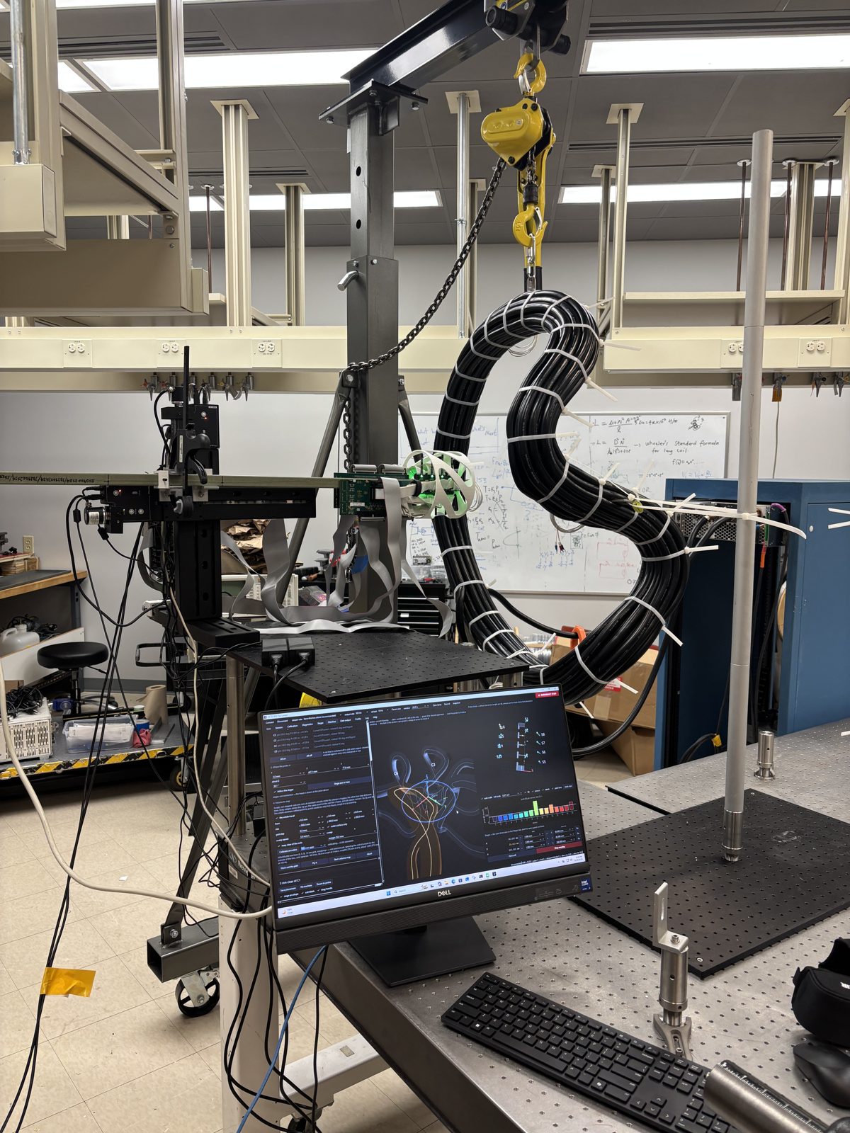
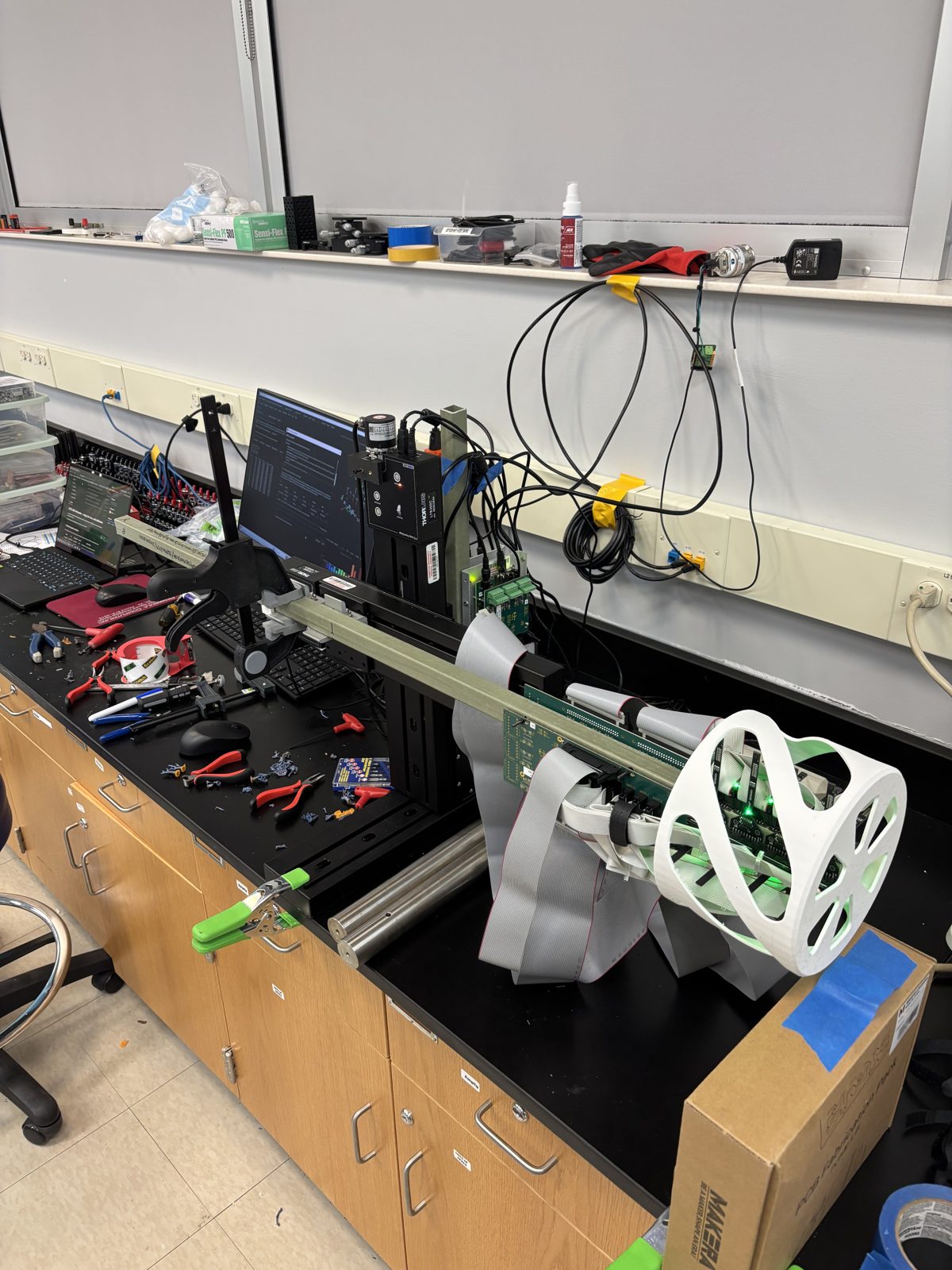
The head is a one-inch square tube carrying sixteen SENIS SENM3Dx eval boards, four per face, each chip at the tip of a 92 mm arm. Every chip measures Bx, By and Bz plus its own virtual-ground reference, which turned out to be the key diagnostic: noise on a field channel and its reference means the cable; noise on the field channel alone means the chip.
Two D-TACQ ACQ1001 carriers digitise all 64 channels at 200 kSPS over gigabit Ethernet. Only one of them has quadrature-encoder logic in its FPGA, which is where the three stage encoders go.
From a box of parts to a field map
Two boxes, not one
Imported the bench tooling and found why only 32 channels ever showed up: there are two digitisers. Harmonised all 16 chips to gain 3000 (±20 mT), cut Connect from 85 s to 10 s and the live repaint from 39 s to 22 ms.
Motors
Three Thorlabs LTS300C stages on the bus, axis map recorded, the reverse-mounted z axis handled once in stages.json so no map is ever silently mirrored.
Encoders and bad chips
The z encoder counted 14,400 counts/mm and agreed with the stage to 0.3 µm over 20 mm. Swapping two eval kits proved the noisy channels travel with the chip, not the cable.
The magnet tells the truth
The guided magnet run measured where every sensor actually sits. Twelve of sixteen were where the drawing said; one whole face ran backwards along the tube. Latching emergency stop added the same day.
Restructure
Split into an installable package with tabs, a test suite and CI, and added the Machine tab: the simsopt coil set in 3D with live clearance to the windings.
Into the coils
Volumes swept instead of rastered, with position latched in the frame. The gantry moved to the energised STAR_Lite coils and mapped through the night.
Let the magnet measure the probe
Holding a magnet up to each sensor by hand gives a different distance every time, and a dipole falls off as 1/r³: a 10% distance error is a 30% amplitude error. Correcting for it needs the geometry, which is exactly what is not yet known.
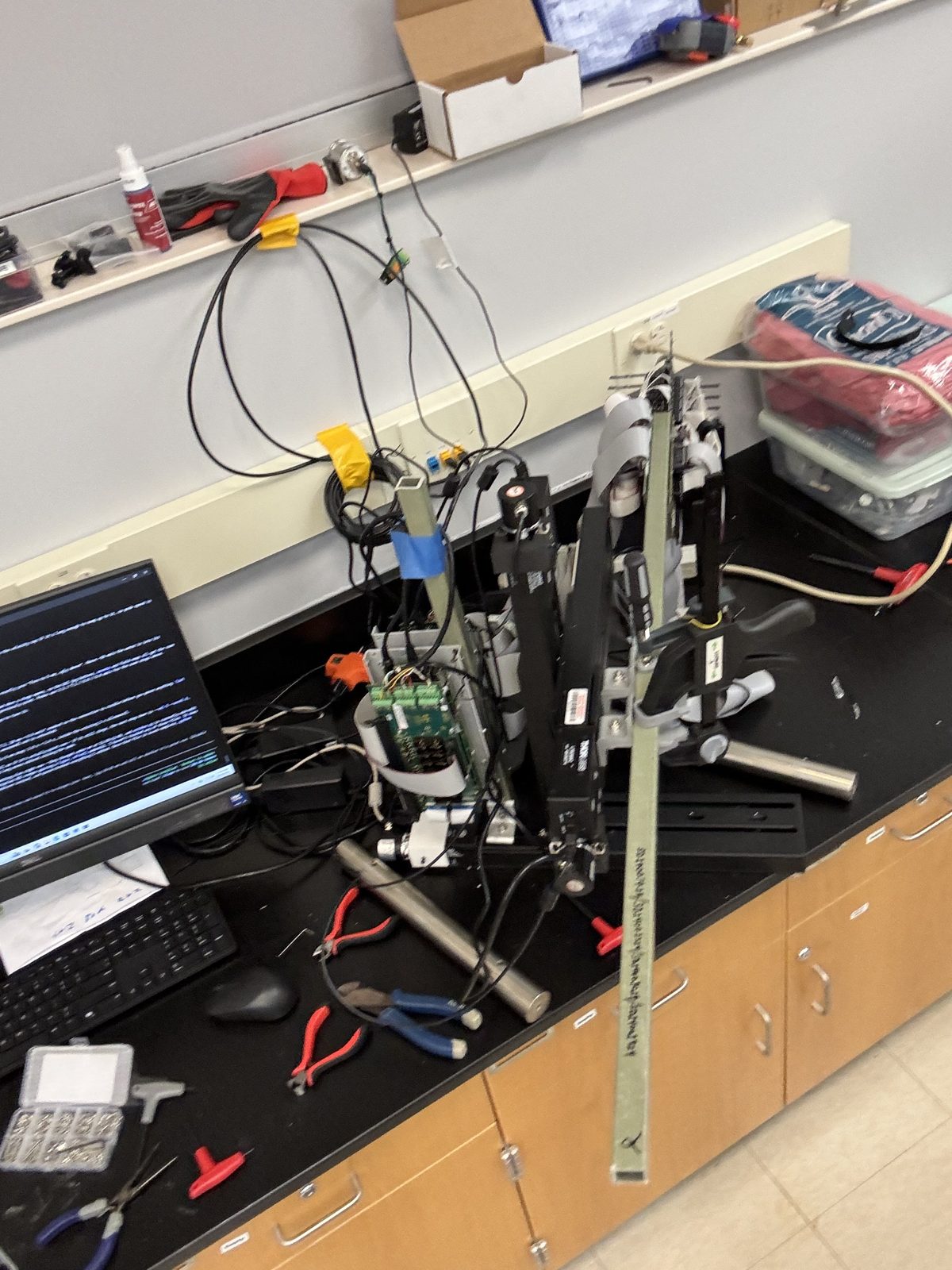
With motors the geometry cancels instead. The head drives along its own axis past a fixed magnet, so the four sensors of a face pass at the same closest approach. A quarter turn, and the next face gets its go. Four poses later every peak is directly comparable, and the run also revealed that one face had been mounted backwards.
Every sensor on a face passes the magnet at the same closest approach, so the peaks differ only by gain: trim = median(peak) / peak. Peak values shown are from the first real guided run.
Sweep, don't raster
Move, stop, settle, average is the right way to measure one point. For a volume it is an impossible experiment. So the mapper sweeps one axis at constant velocity while the stream logs continuously and steps the other two between lines, cutting every line back to the space the whole probe body actually fits in between the coils.
300 mm cube on a 10 mm grid: 29,791 points × 7.5 s ≈ 62 hours.
The same 29,791 samples come off a 300 mm line in 30 s. Lines always run in +y, the dashed return keeps leadscrew backlash out of the map.
Encoders buy you when, not where
The stage controllers report position over USB from a cache refreshed every 100 ms, on the PC's clock, while the field arrives on the digitiser's clock. At sweep speed that mismatch smears every sample by about a millimetre, randomly.
The rotary encoders count the same leadscrew, so they are no more accurate. What they give is timing: their count is latched into the very ADC frame it belongs to. Measured: 14,400 counts/mm, 0.3 µm disagreement over a 20 mm move, no dropped counts up to 12 mm/s.
How sensitive is it really?
At gain 3000 the sensors are at their most sensitive setting. Resolution is then set by noise, which is white: average 100× longer and it drops 10×. The clean sensors track the datasheet almost exactly, from 62 µT at full bandwidth down to 0.7 µT at 10 Hz.
Below about 1 Hz the curve flattens at the chips' offset drift, roughly 1 µT per axis: about 2% of Earth's field, enough to see the probe turn.
Energising the coils
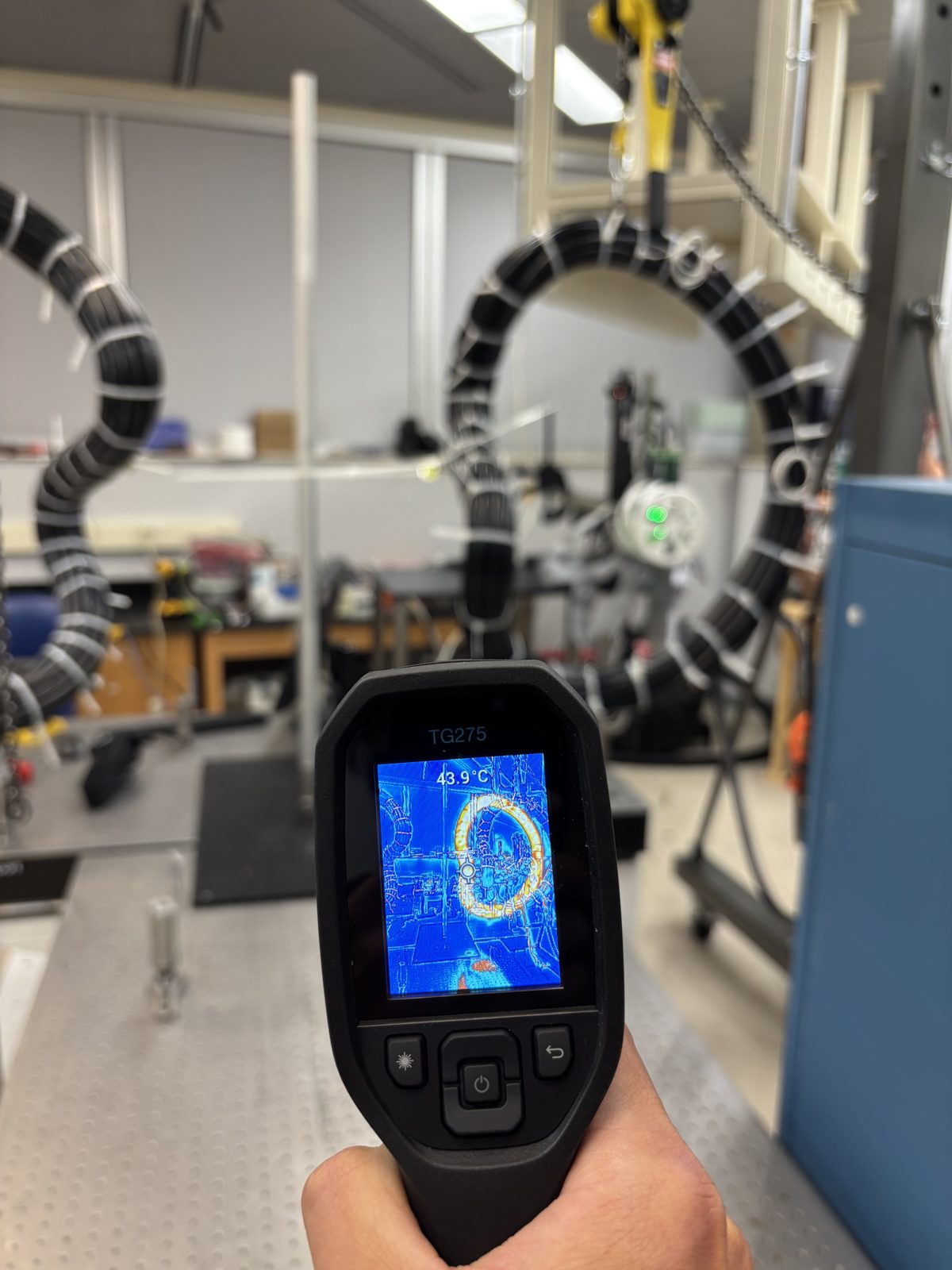
The last nights of August were spent at the coils: positioning the probe against the simsopt model, checking clearance against 60 mm conductor packs, watching the winding temperature, and letting the gantry sweep.
- •16 SENIS 3D Hall sensors, 48 field channels, 200 kSPS per channel
- •Three Thorlabs LTS300C stages spanning a 300 mm cube
- •Quadrature encoders latched in the same ADC frame as the field
- •Swept volume maps instead of stop-and-settle rasters
- •Guided-magnet calibration that cancels the probe geometry
- •3D machine view of the simsopt coil set with live clearance
- •Latching emergency stop and explicit position trust
- •Two unsynchronised digitisers with different frame layouts
- •Telling a bad Hall chip from a bad cable without unplugging anything
- •USB position readouts that were 0–100 ms stale while moving
- •A reverse-mounted z axis that would silently mirror every map
- •Keeping a 159 mm probe out of 60 mm coil windings
- •Synchronism, not accuracy, is what encoders buy you on a leadscrew
- •A settled raster of a volume is an impossible experiment; a sweep is not
- •Measure the geometry with the instrument rather than trusting the drawing
- •Short throughput tests understate a stream that ramps for 30 s
More from the bench
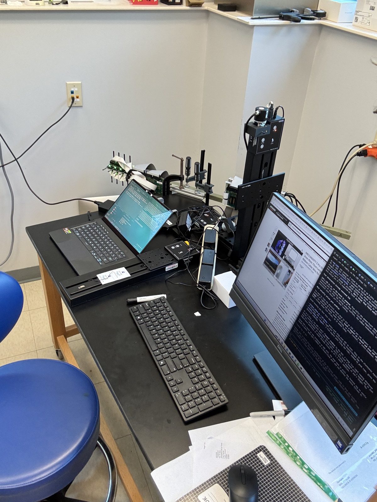
Day one: the gantry, the probe and a lot of terminals
Bolting the three LTS300C stages into a cartesian gantry
Late-night commissioning, all sixteen sensors lit up
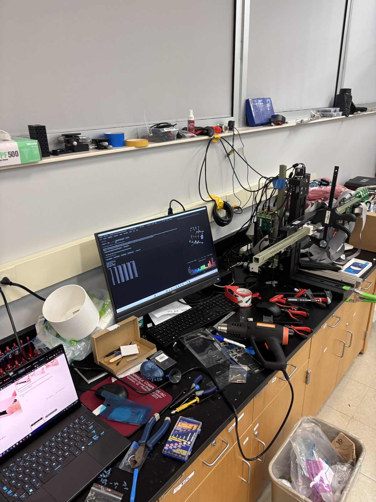
Calibration day: live sensor bars on screen, heat gun on standby
The probe head in its printed cage, ready to travel to the coils
Gantry parked beside the STAR_Lite coils, machine view on screen
Keeping an eye on the energised coil: 43.9 °C on the windings
The low-tech field check: a steel chain leaning into the energised coil
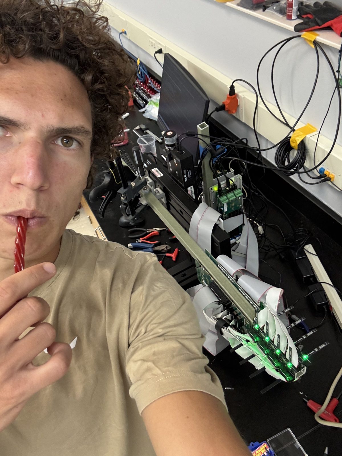
The head sweeping on the bench with all sensors streaming
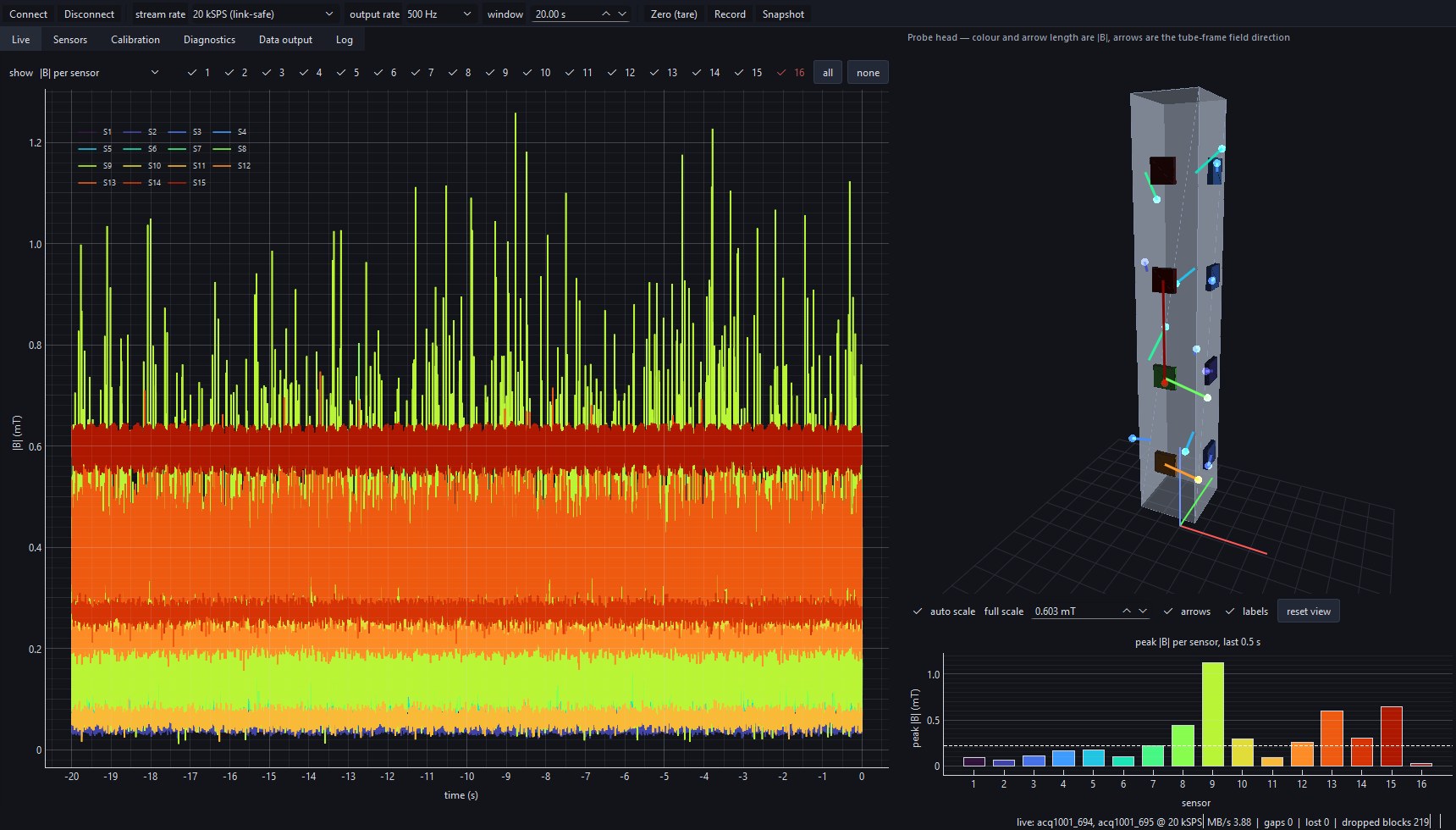
Live view on real hardware: |B| per sensor, 3D head and peak bars
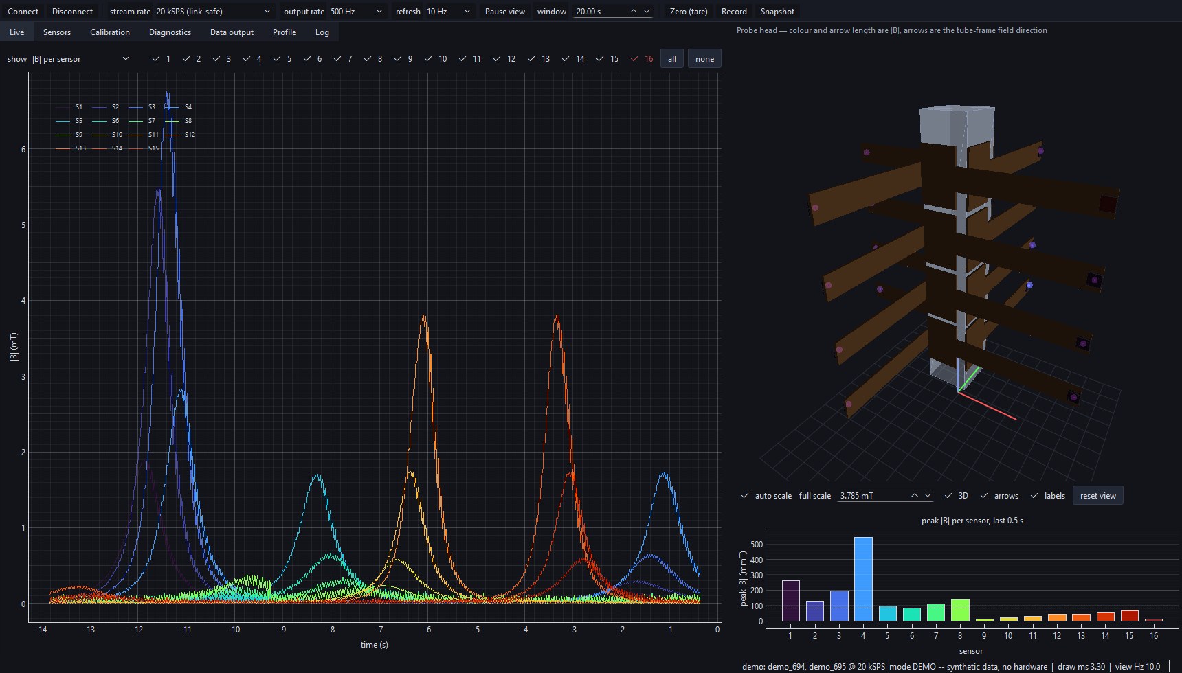
A magnet pass: four rings of sensors peaking one after another